Material docente en Quarto a partir del script original
Autores/as
Sergi Ramírez
Dante Conti
1 Introducción
Este documento docente presenta, de forma estructurada y comentada, distintos métodos de imputación de datos faltantes en R.
Se ha respetado al máximo la organización del script original, incorporando:
explicación conceptual antes de cada bloque,
comentarios detallados dentro del código,
separación por apartados para facilitar la docencia,
y una estructura adecuada para usar directamente en Quarto.
1.1 Objetivos docentes
Al finalizar este material, el estudiante debería poder:
generar artificialmente valores perdidos,
explorar patrones de missingness,
distinguir entre técnicas básicas y avanzadas de imputación,
aplicar métodos como media, aregImpute, MI, MICE, KNN y missForest,
comparar distribuciones originales e imputadas.
2 Carga de librerías
En este primer bloque cargamos todos los paquetes necesarios para trabajar con visualización, exploración de valores perdidos e imputación.
# Carreguem les llibreries =====================================================# Vector con los paquetes que vamos a necesitar durante toda la práctica.# Incluye paquetes para:# - visualización (ggplot2, plotly, visdata, VIM)# - manipulación de datos (dplyr, tidyverse)# - análisis de missingness (naniar, mi)# - imputación (Hmisc, mice, DMwR, missForest)list.of.packages <-c("ggplot2", "plotly", "dplyr", "tidyverse", "naniar","mi", "Hmisc", "mice", "pool", "VIM", "missForest", "RANN", "caret")# Detectamos qué paquetes no están instalados en el sistema.new.packages <- list.of.packages[!(list.of.packages %in%installed.packages()[, "Package"])]# Si falta alguno, lo instalamos automáticamente.if (length(new.packages) >0) {install.packages(new.packages)}# Cargamos todos los paquetes en memoria.lapply(list.of.packages, require, character.only =TRUE)
# Limpiamos objetos auxiliares que ya no necesitamos y lanzamos el recolector# de basura para liberar memoria.rm(list.of.packages, new.packages)gc()
          used  (Mb) gc trigger  (Mb) max used  (Mb)
Ncells 3625439 193.7    7357892 393.0  4386978 234.3
Vcells 6067688  46.3   10146329  77.5  8360610  63.8
3 Generación de datos con valores perdidos
Para practicar métodos de imputación, primero generamos una versión incompleta del conjunto de datos iris, introduciendo un 10% de valores ausentes de forma artificial.
# Generate data with NA's ======================================================# Generamos una copia del dataset iris con aproximadamente un 10% de valores NA.# La función prodNA del paquete missForest introduce missing values de forma# artificial para que podamos practicar imputación.iris.mis <- missForest::prodNA(iris, noNA =0.1)# Otras formas de crear valores ausentes artificialmente en un dataframe:# iris.mis <- mi::create.missing(iris, pct.mis = 10)# Mostramos un resumen básico del dataset con NA para inspeccionar su estructura.summary(iris.mis)
  Sepal.Length    Sepal.Width     Petal.Length    Petal.Width
 Min.   :4.300   Min.   :2.000   Min.   :1.000   Min.   :0.100
 1st Qu.:5.100   1st Qu.:2.800   1st Qu.:1.600   1st Qu.:0.300
 Median :5.700   Median :3.000   Median :4.300   Median :1.300
 Mean   :5.796   Mean   :3.065   Mean   :3.726   Mean   :1.168
 3rd Qu.:6.350   3rd Qu.:3.400   3rd Qu.:5.100   3rd Qu.:1.800
 Max.   :7.700   Max.   :4.400   Max.   :6.900   Max.   :2.500
 NA's   :11      NA's   :17      NA's   :13      NA's   :15
       Species
 setosa    :44
 versicolor:45
 virginica :42
 NA's      :19
4 Little Test
Una cuestión importante en datos faltantes es entender si los NA aparecen completamente al azar o siguen algún patrón. Para ello usamos el test MCAR.
# Little Test ==================================================================# Aplicamos el test MCAR (Missing Completely At Random).# Este contraste ayuda a evaluar si los datos faltantes se generan de manera# completamente aleatoria.naniar::mcar_test(iris.mis)
# Interpretación conceptual:# - Si el p-valor es pequeño, rechazamos que los missing sean completamente aleatorios.# - Si el p-valor no es pequeño, no tenemos evidencia para rechazar MCAR.# Nota importante docente:# En el script original aparece el comentario:# "If the test p-value is less than 0 this means..."# Lo correcto estadísticamente sería hablar de un p-valor bajo, por ejemplo < 0.05.
5 Patrones descriptivos de valores perdidos en una base de datos
Antes de imputar, conviene visualizar y describir los patrones de ausencia. Esto ayuda a detectar si hay variables particularmente afectadas o relaciones entre missingness y otras variables.
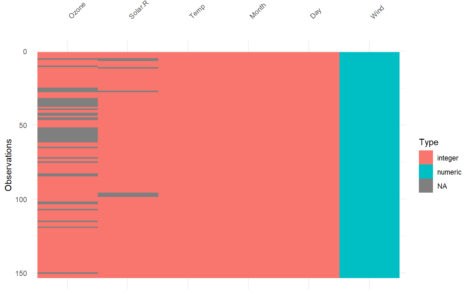
5.1 Exploración visual de missingness
# Descriptive NA's patterns in a databases =====================================# Cargamos explícitamente visdat para sus funciones de visualización.library(visdat)# Visualizamos el tipo de dato y la presencia de NA en airquality.vis_dat(airquality)
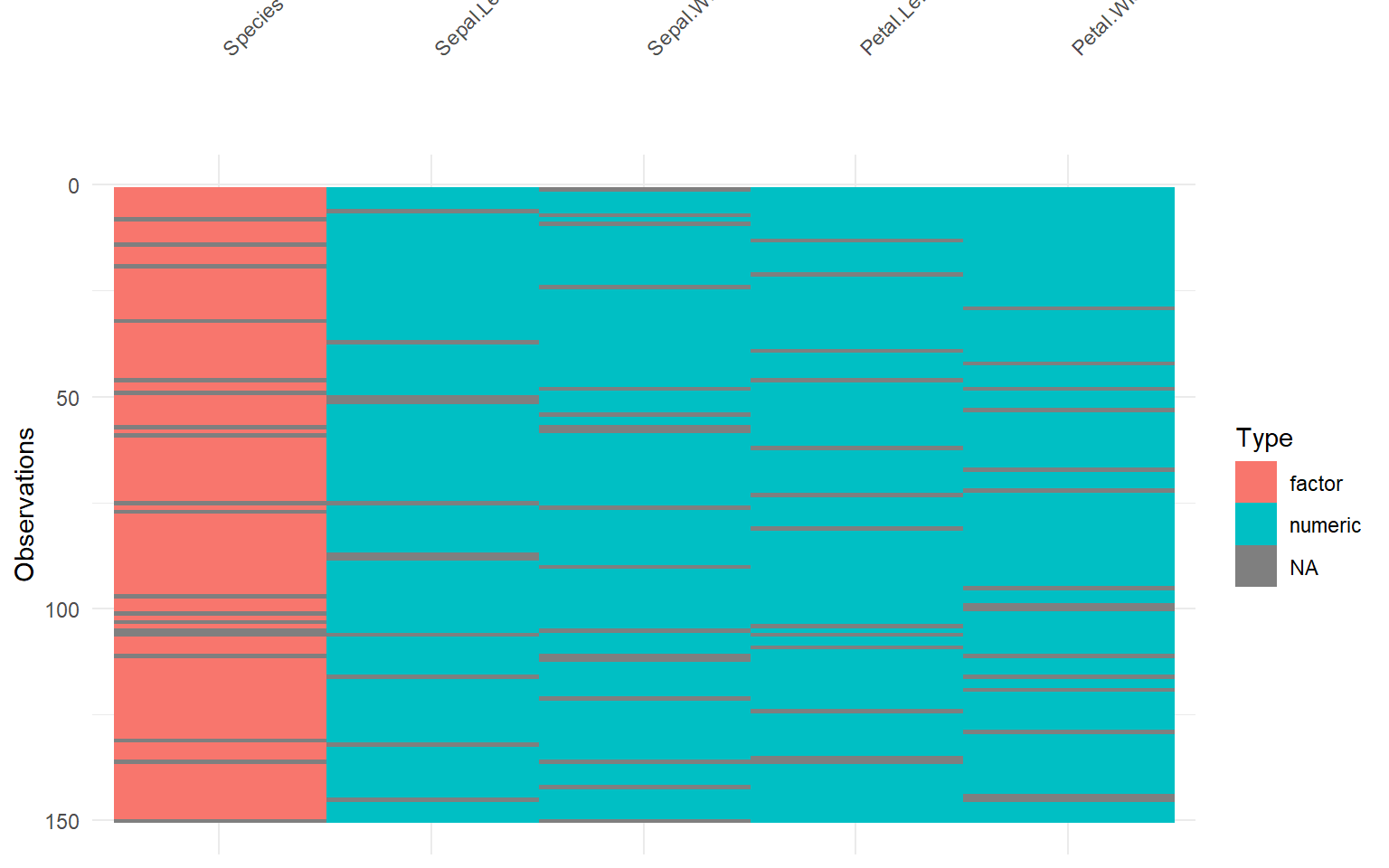
# Visualizamos el tipo de dato y la presencia de NA en iris.mis.vis_dat(iris.mis)
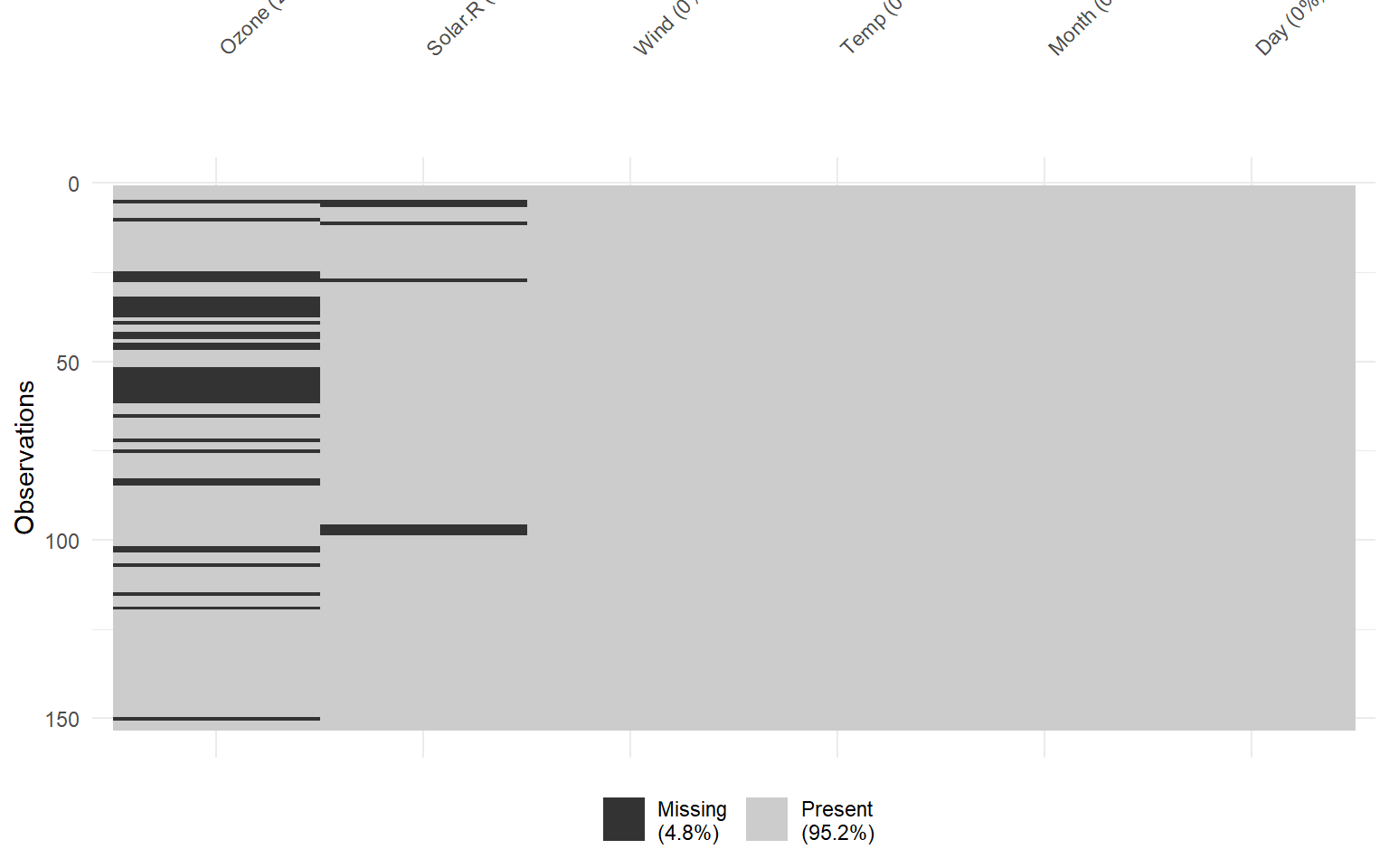
# Representación específica de valores perdidos en airquality.vis_miss(airquality)
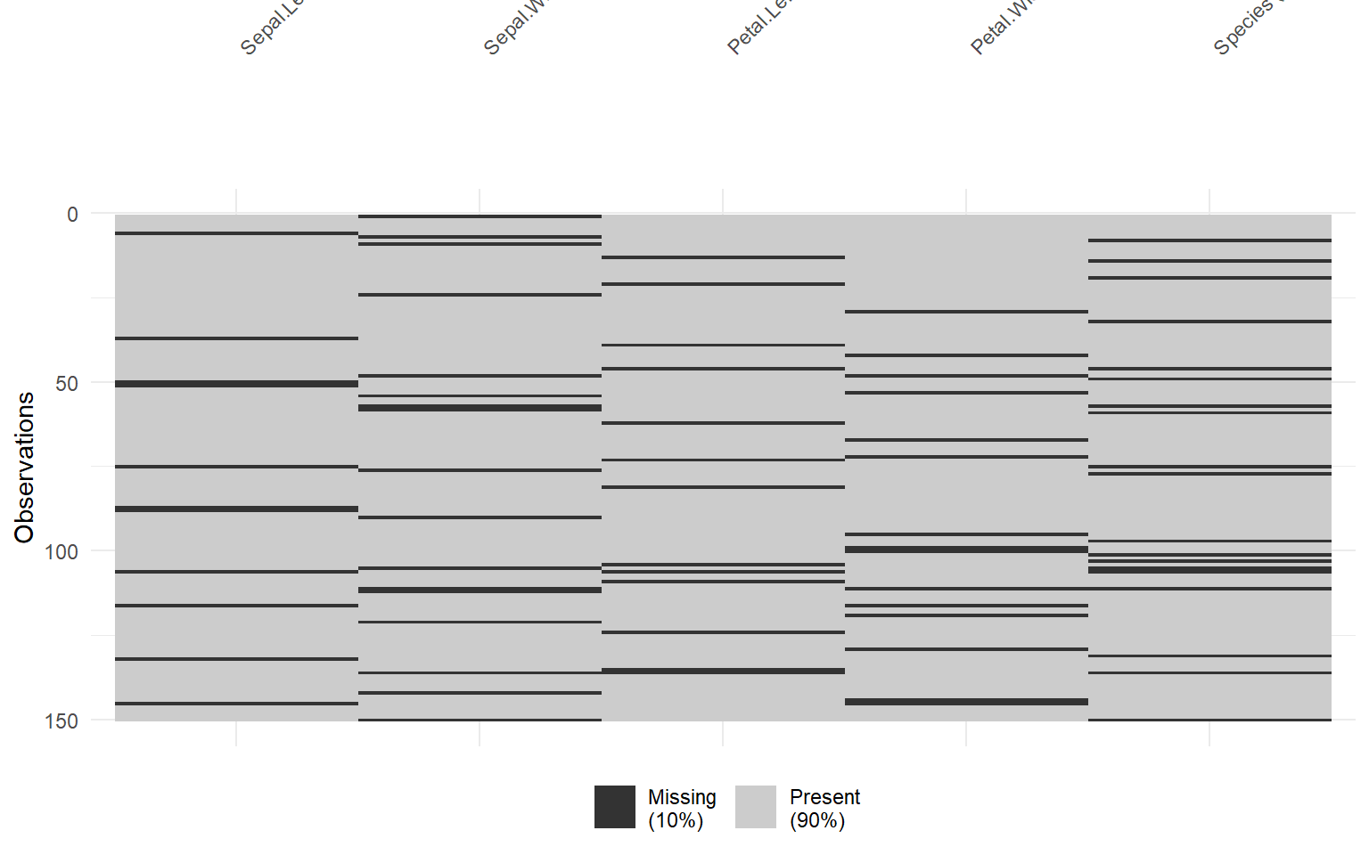
# Representación específica de valores perdidos en iris.mis.vis_miss(iris.mis)
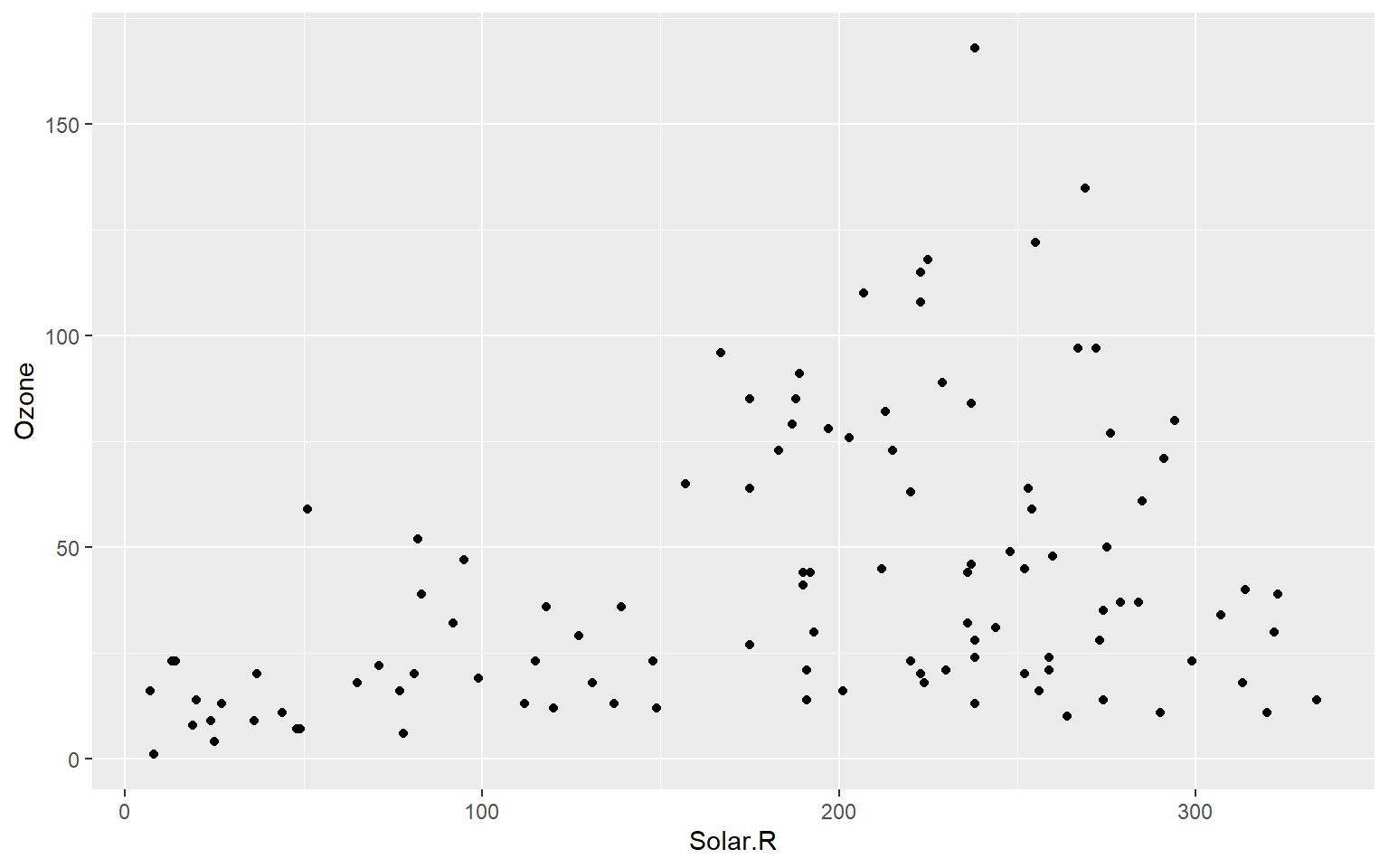
5.2 Relación entre valores perdidos y variables numéricas
# Gráfico básico de dispersión sin destacar missingness.ggplot(airquality, aes(x = Solar.R, y = Ozone)) +geom_point()
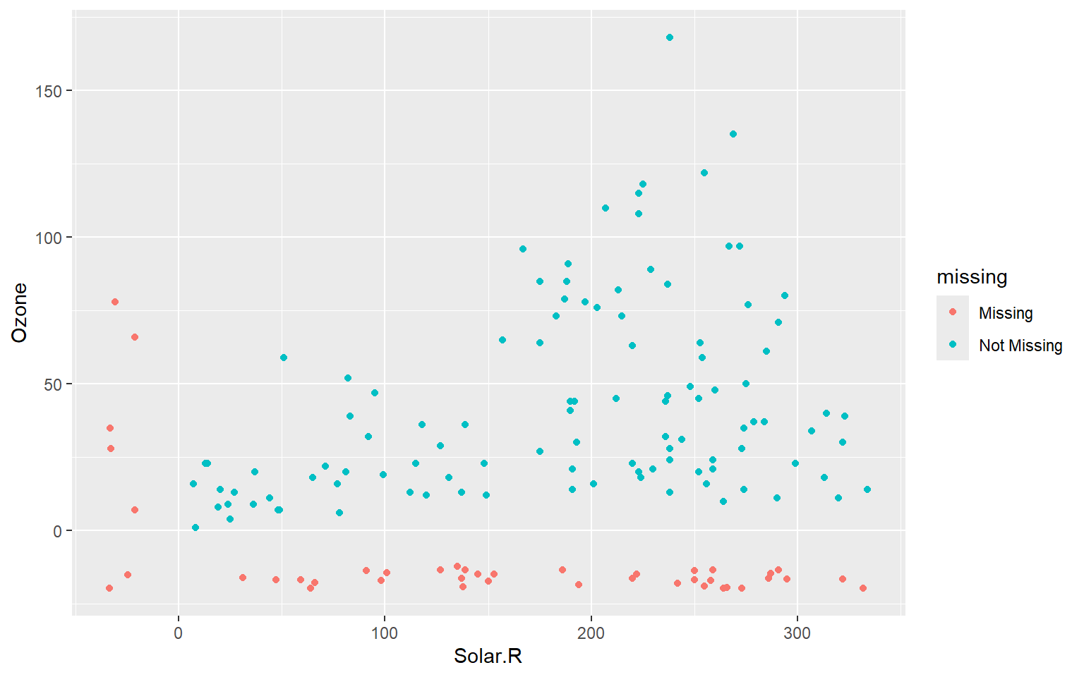
# Gráfico de dispersión destacando las observaciones con missingness.ggplot(airquality, aes(x = Solar.R, y = Ozone)) +geom_miss_point()
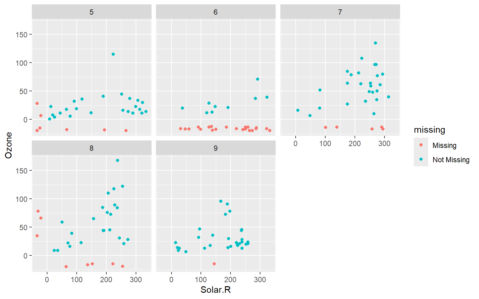
# Añadimos facetado por mes para observar si el patrón de NA cambia según el mes.ggplot(airquality, aes(x = Solar.R, y = Ozone)) +geom_miss_point() +facet_wrap(~Month)
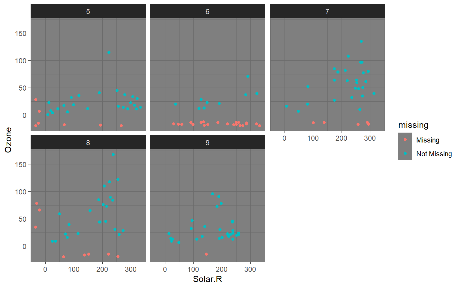
# Mismo gráfico anterior pero con tema oscuro para enfatizar la visualización.ggplot(airquality, aes(x = Solar.R, y = Ozone)) +geom_miss_point() +facet_wrap(~Month) +theme_dark()
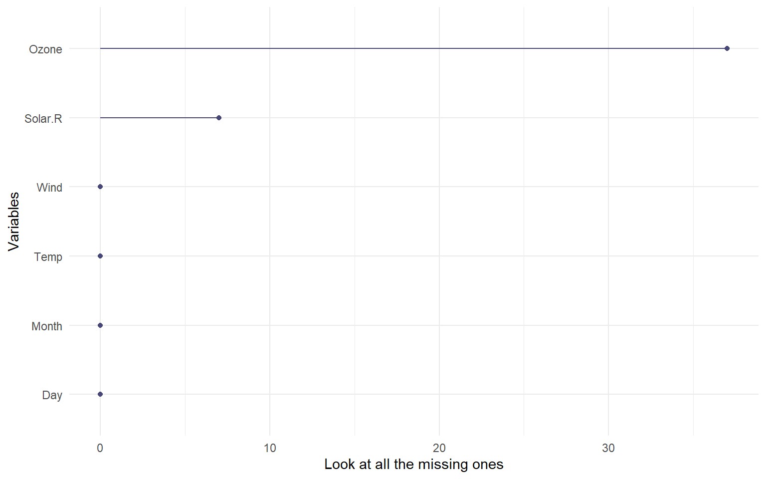
5.3 Visualización del número de missings por variable
# Visualizamos cuántos NA tiene cada variable.gg_miss_var(airquality) +labs(y ="Look at all the missing ones")
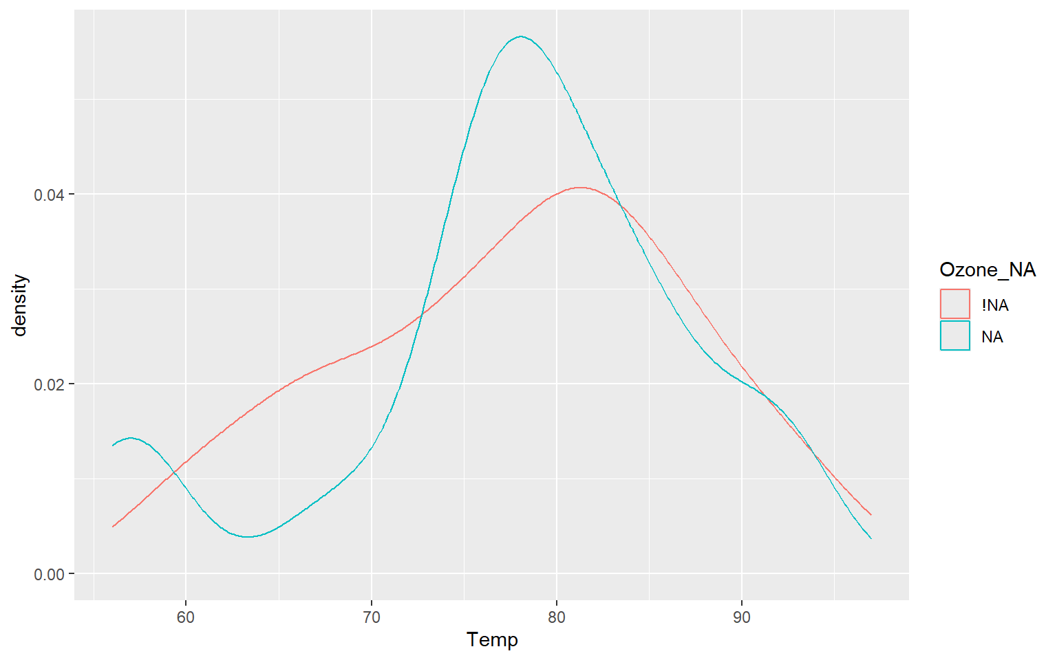
5.4 Sombra de missingness y resumen por grupos
# Detect NA in Dataframe =======================================================# Creamos un shadow matrix: añade variables auxiliares con sufijo _NA que indican# si el valor original era NA o no.aq_shadow <-bind_shadow(airquality)# Calculamos estadísticas descriptivas de Solar.R separando los registros según# si Ozone es NA o no.airquality %>%bind_shadow() %>%group_by(Ozone_NA) %>%summarise_at(.vars ="Solar.R",.funs =c("mean", "sd", "var", "min", "max"),na.rm =TRUE )
# Representamos la distribución de la temperatura diferenciando los casos en los# que Ozone está ausente de aquellos en los que no lo está.ggplot(aq_shadow, aes(x = Temp, colour = Ozone_NA)) +geom_density()
5.5 Estadísticos de missingness
# Extract statistics with NAs in Data Frame ====================================# Proporción de casos (filas) que contienen algún NA.prop_miss_case(airquality)
[1] 0.2745098
# Porcentaje de casos con NA.pct_miss_case(airquality)
[1] 27.45098
# Resumen por fila del patrón de missingness.miss_case_summary(airquality)
# Tabla de frecuencia del número de missings por fila.miss_case_table(airquality)
# Proporción de missings por variable.prop_miss_var(airquality)
[1] 0.3333333
# Porcentaje de missings por variable.pct_miss_var(airquality)
[1] 33.33333
# Resumen de missingness por variable.miss_var_summary(airquality)
# Tabla de frecuencia de missings por variable.miss_var_table(airquality)
6 1.1 Imputación básica
En este apartado se ilustran técnicas sencillas de imputación, útiles para comprender la lógica general aunque normalmente insuficientes en contextos reales complejos.
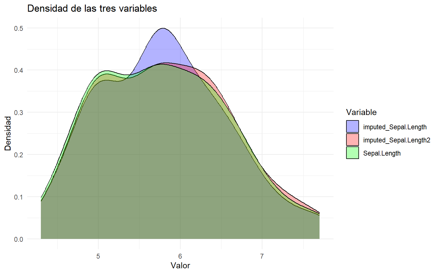
6.1 Imputación con la media y con valores aleatorios
# 1.1 Basic Imputation ========================================================# Imputamos los NA de Sepal.Length usando la media de la variable.# La función impute del paquete Hmisc devuelve una versión imputada de la variable.iris.mis[, "imputed_Sepal.Length"] <-with(iris.mis, impute(Sepal.Length, mean))# Imputamos los NA de Sepal.Length usando valores aleatorios observados.iris.mis[, "imputed_Sepal.Length2"] <-with(iris.mis, impute(Sepal.Length, "random"))# Nota docente:# De forma análoga se podrían usar estrategias como min, max o median.# Reestructuramos los datos a formato largo para comparar distribuciones.df_long <- iris.mis %>%select(Sepal.Length, imputed_Sepal.Length, imputed_Sepal.Length2) %>%pivot_longer(cols =everything(), names_to ="Variable", values_to ="Valor")# Representamos la densidad de la variable original y de las variables imputadas.ggplot(df_long, aes(x = Valor, fill = Variable)) +geom_density(alpha =0.3) +labs(title ="Densidad de las tres variables",x ="Valor",y ="Densidad" ) +theme_minimal() +scale_fill_manual(values =c("blue", "red", "green"))
# Eliminamos las variables auxiliares para no contaminar el dataframe original.iris.mis[, c("imputed_Sepal.Length", "imputed_Sepal.Length2")] <-NULL
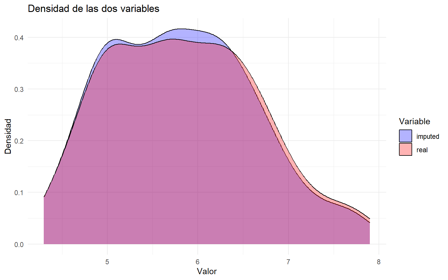
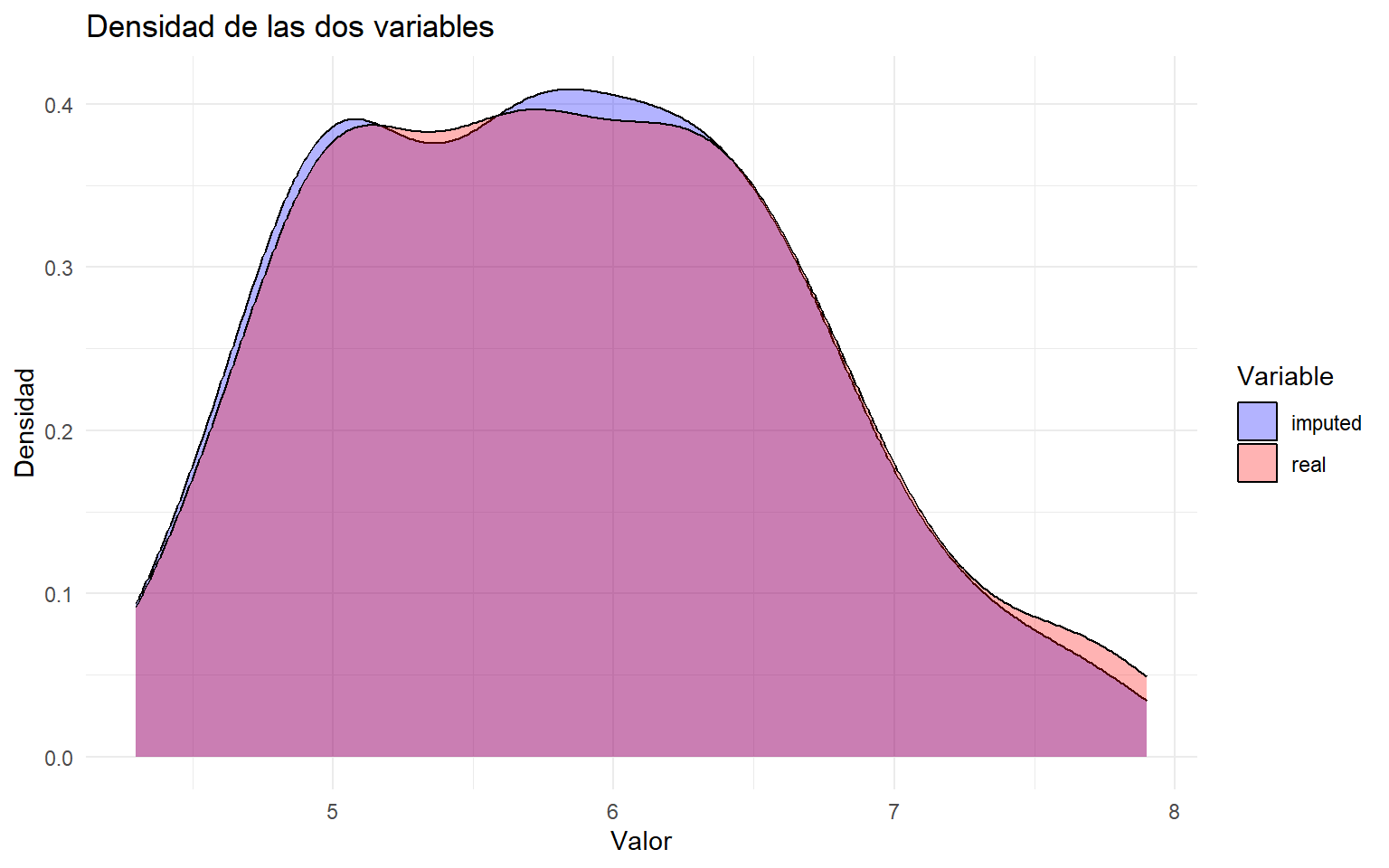
6.2 Imputación con aregImpute
aregImpute implementa una imputación basada en modelos aditivos flexibles y múltiples simulaciones. Aquí se aplica sobre todas las variables del dataset.
# ------------------------------------------------------------------------------# using argImpute# Ajustamos el modelo de imputación.# n.impute = 5 indica que se generan 5 imputaciones para los valores ausentes.impute_arg <-aregImpute(~ Sepal.Length + Sepal.Width + Petal.Length + Petal.Width + Species,data = iris.mis,n.impute =5)
# Mostramos el objeto resultante para inspeccionar la imputación.impute_arg
Multiple Imputation using Bootstrap and PMM

aregImpute(formula = ~Sepal.Length + Sepal.Width + Petal.Length +
    Petal.Width + Species, data = iris.mis, n.impute = 5)

n: 150  p: 5    Imputations: 5      nk: 3

Number of NAs:
Sepal.Length  Sepal.Width Petal.Length  Petal.Width      Species
          11           17           13           15           19

             type d.f.
Sepal.Length    s    2
Sepal.Width     s    2
Petal.Length    s    2
Petal.Width     s    2
Species         c    2

Transformation of Target Variables Forced to be Linear

R-squares for Predicting Non-Missing Values for Each Variable
Using Last Imputations of Predictors
Sepal.Length  Sepal.Width Petal.Length  Petal.Width      Species
       0.855        0.621        0.979        0.962        0.989
# Revisamos específicamente las imputaciones generadas para Sepal.Length.impute_arg$imputed$Sepal.Length
# Calculamos la media de las 5 imputaciones para cada observación ausente.imputed_Sepal.Length <-rowMeans(impute_arg$imputed$Sepal.Length)# Creamos una nueva variable partiendo de la variable real original.new_var_imputed <- iris$Sepal.Length# Sustituimos únicamente las posiciones que tenían NA por la media imputada.new_var_imputed[as.numeric(names(imputed_Sepal.Length))] <- imputed_Sepal.Length# Comparamos la distribución real frente a la imputada.newBD <-data.frame(real = iris[, "Sepal.Length"], imputed = new_var_imputed)df_long <- newBD %>%pivot_longer(cols =everything(), names_to ="Variable", values_to ="Valor")ggplot(df_long, aes(x = Valor, fill = Variable)) +geom_density(alpha =0.3) +labs(title ="Densidad de las dos variables",x ="Valor",y ="Densidad" ) +theme_minimal() +scale_fill_manual(values =c("blue", "red"))
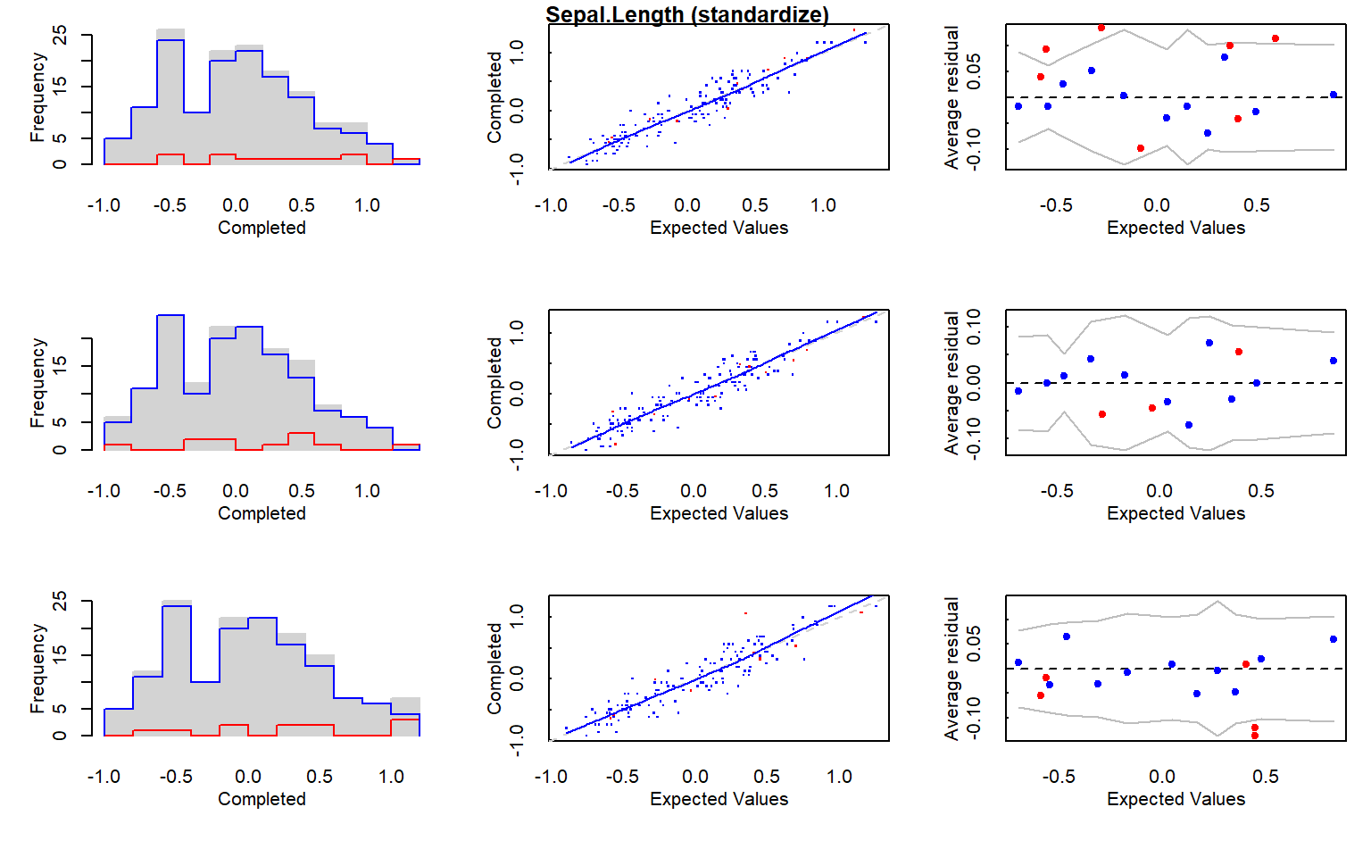
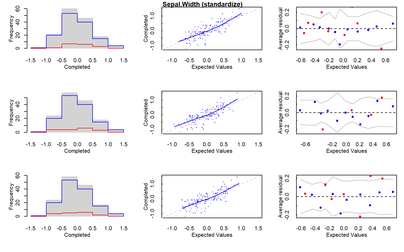
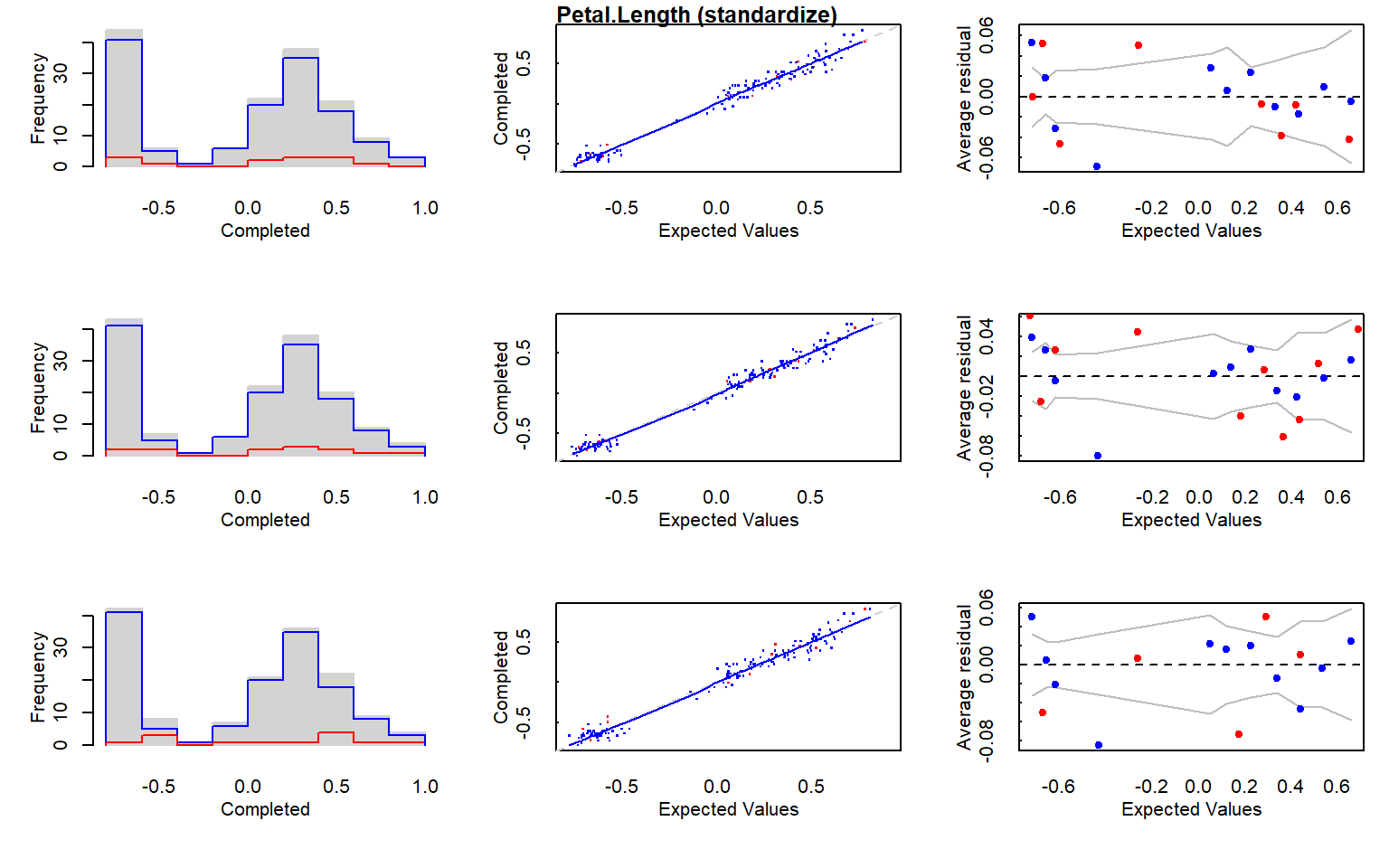
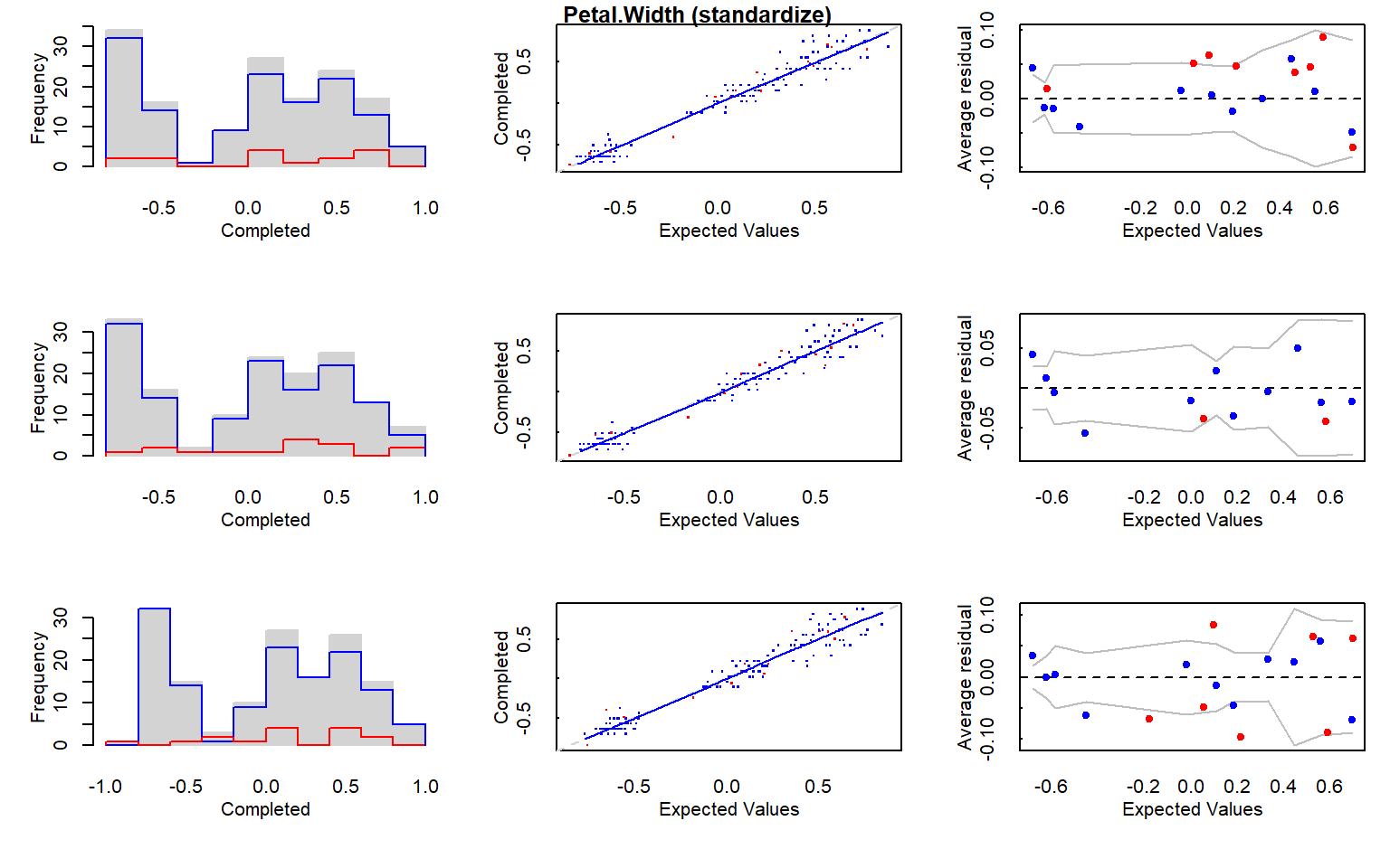
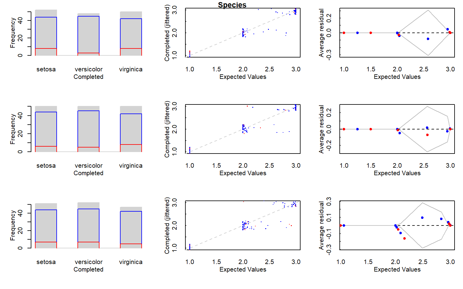
Este bloque usa el paquete mi, que implementa imputación múltiple mediante aproximaciones iterativas basadas en modelos probabilísticos.
# 1.1.1 Multiple Iterative Regression Imputation (MI method) -------------------# Ejecutamos la imputación múltiple con una semilla fija para garantizar# reproducibilidad.mi_data <-mi(iris.mis, seed =335)# Resumen del modelo de imputación.summary(mi_data)
$Sepal.Length
$Sepal.Length$is_missing
missing
FALSE  TRUE
  139    11

$Sepal.Length$imputed
   Min. 1st Qu.  Median    Mean 3rd Qu.    Max.
-0.8313 -0.1808  0.3217  0.2455  0.6659  1.3929

$Sepal.Length$observed
    Min.  1st Qu.   Median     Mean  3rd Qu.     Max.
-0.92667 -0.43102 -0.05928  0.00000  0.37441  1.17984


$Sepal.Width
$Sepal.Width$is_missing
missing
FALSE  TRUE
  133    17

$Sepal.Width$imputed
    Min.  1st Qu.   Median     Mean  3rd Qu.     Max.
-0.91754 -0.32512  0.05625  0.03350  0.40277  0.99748

$Sepal.Width$observed
   Min. 1st Qu.  Median    Mean 3rd Qu.    Max.
-1.1920 -0.2963 -0.0724  0.0000  0.3755  1.4951


$Petal.Length
$Petal.Length$is_missing
missing
FALSE  TRUE
  137    13

$Petal.Length$imputed
    Min.  1st Qu.   Median     Mean  3rd Qu.     Max.
-0.77755 -0.50058  0.27530  0.08156  0.43277  0.90765

$Petal.Length$observed
   Min. 1st Qu.  Median    Mean 3rd Qu.    Max.
-0.7797 -0.6081  0.1643  0.0000  0.3932  0.9081


$Petal.Width
$Petal.Width$is_missing
missing
FALSE  TRUE
  135    15

$Petal.Width$imputed
   Min. 1st Qu.  Median    Mean 3rd Qu.    Max.
-0.8516 -0.1801  0.1935  0.1346  0.5115  0.8273

$Petal.Width$observed
    Min.  1st Qu.   Median     Mean  3rd Qu.     Max.
-0.70623 -0.57400  0.08718  0.00000  0.41776  0.88058


$Species
$Species$crosstab

             observed imputed
  setosa          176      27
  versicolor      180      22
  virginica       168      27
# Gráficos diagnósticos del proceso de imputación.plot(mi_data)
# Evitamos que R pregunte entre gráficos cuando hay múltiples paneles.par(ask =FALSE)# Revisamos la estructura interna del objeto de imputación.mi_data@data
$`chain:1`
Object of class missing_data.frame with 150 observations on 5 variables

There are 14 missing data patterns

Append '@patterns' to this missing_data.frame to access the corresponding pattern for every observation or perhaps use table()

                              type missing method  model
Sepal.Length            continuous      11    ppd linear
Sepal.Width             continuous      17    ppd linear
Petal.Length            continuous      13    ppd linear
Petal.Width             continuous      15    ppd linear
Species      unordered-categorical      19    ppd mlogit

                  family     link transformation
Sepal.Length    gaussian identity    standardize
Sepal.Width     gaussian identity    standardize
Petal.Length    gaussian identity    standardize
Petal.Width     gaussian identity    standardize
Species      multinomial    logit           <NA>

$`chain:2`
Object of class missing_data.frame with 150 observations on 5 variables

There are 14 missing data patterns

Append '@patterns' to this missing_data.frame to access the corresponding pattern for every observation or perhaps use table()

                              type missing method  model
Sepal.Length            continuous      11    ppd linear
Sepal.Width             continuous      17    ppd linear
Petal.Length            continuous      13    ppd linear
Petal.Width             continuous      15    ppd linear
Species      unordered-categorical      19    ppd mlogit

                  family     link transformation
Sepal.Length    gaussian identity    standardize
Sepal.Width     gaussian identity    standardize
Petal.Length    gaussian identity    standardize
Petal.Width     gaussian identity    standardize
Species      multinomial    logit           <NA>

$`chain:3`
Object of class missing_data.frame with 150 observations on 5 variables

There are 14 missing data patterns

Append '@patterns' to this missing_data.frame to access the corresponding pattern for every observation or perhaps use table()

                              type missing method  model
Sepal.Length            continuous      11    ppd linear
Sepal.Width             continuous      17    ppd linear
Petal.Length            continuous      13    ppd linear
Petal.Width             continuous      15    ppd linear
Species      unordered-categorical      19    ppd mlogit

                  family     link transformation
Sepal.Length    gaussian identity    standardize
Sepal.Width     gaussian identity    standardize
Petal.Length    gaussian identity    standardize
Petal.Width     gaussian identity    standardize
Species      multinomial    logit           <NA>

$`chain:4`
Object of class missing_data.frame with 150 observations on 5 variables

There are 14 missing data patterns

Append '@patterns' to this missing_data.frame to access the corresponding pattern for every observation or perhaps use table()

                              type missing method  model
Sepal.Length            continuous      11    ppd linear
Sepal.Width             continuous      17    ppd linear
Petal.Length            continuous      13    ppd linear
Petal.Width             continuous      15    ppd linear
Species      unordered-categorical      19    ppd mlogit

                  family     link transformation
Sepal.Length    gaussian identity    standardize
Sepal.Width     gaussian identity    standardize
Petal.Length    gaussian identity    standardize
Petal.Width     gaussian identity    standardize
Species      multinomial    logit           <NA>
8 1.1.2 Media condicionada por variable objetivo
Aquí se aplica una estrategia simple pero útil en docencia: imputar con la media del grupo, definida por una variable objetivo o categórica, en este caso Species.
# 1.1.2 MEAN WITH TARGET VARS --------------------------------------------------# Definimos la variable objetivo o de agrupación.target <-"Species"# Construimos un dataset sin la variable target para introducir NA únicamente# en las variables predictoras.data <-subset(iris, select =-c(get(target)))# Generamos valores ausentes de forma artificial.data <-prodNA(data, noNA =0.1)# Recuperamos la variable target original.data$Species <- iris[, target]# Identificamos qué variables debemos imputar: todas excepto la target.varImp <-colnames(data)[which(!colnames(data) %in% target)]# Calculamos la media de cada variable numérica dentro de cada grupo de Species.means <-aggregate(data[, varImp], list(data[, target]), mean, na.rm =TRUE)# Imputamos los valores ausentes usando la media de su grupo.for (c in varImp) {for (g in means[, "Group.1"]) {# Condición lógica: filas que pertenecen al grupo g. cond <- data[, target] == g# Detectamos los NA de la variable c dentro de ese grupo. na_index <-is.na(data[, c]) & cond# Sustituimos cada NA por la media del grupo correspondiente. data[na_index, c] <- means[means[, "Group.1"] == g, c] }}# Resumen del dataset imputado.summary(data)
  Sepal.Length    Sepal.Width     Petal.Length    Petal.Width
 Min.   :4.300   Min.   :2.000   Min.   :1.000   Min.   :0.100
 1st Qu.:5.100   1st Qu.:2.800   1st Qu.:1.500   1st Qu.:0.300
 Median :5.900   Median :3.000   Median :4.270   Median :1.326
 Mean   :5.862   Mean   :3.071   Mean   :3.756   Mean   :1.201
 3rd Qu.:6.400   3rd Qu.:3.400   3rd Qu.:5.100   3rd Qu.:1.800
 Max.   :7.900   Max.   :4.400   Max.   :6.900   Max.   :2.500
       Species
 setosa    :50
 versicolor:50
 virginica :50
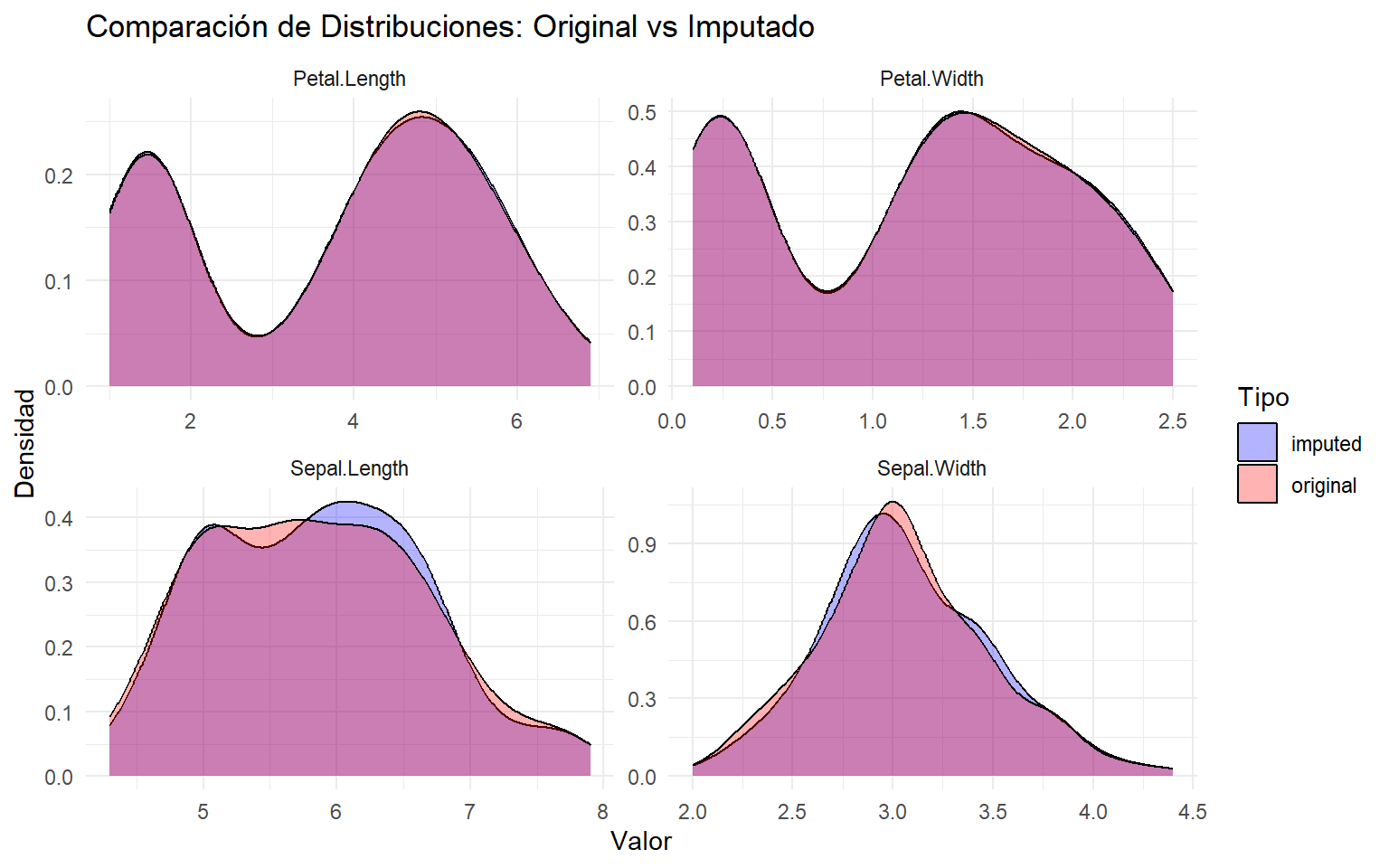
8.1 Comparación visual entre original e imputado
# Marcamos el origen de cada dataset para poder compararlos visualmente.iris[, "Tipo"] <-"original"data[, "Tipo"] <-"imputed"# Fusionamos ambos dataframes en uno solo.data_long <-bind_rows(iris, data)# Seleccionamos únicamente las variables numéricas para representar densidades.cols_numeric <-names(data_long)[sapply(data_long, is.numeric) &names(data_long) !="Tipo"]# Pasamos a formato largo para facetar un gráfico por variable.data_long <- data_long %>%pivot_longer(cols =all_of(cols_numeric), names_to ="Variable", values_to ="Valor")# Representamos la comparación de distribuciones por variable.ggplot(data_long, aes(x = Valor, fill = Tipo)) +geom_density(alpha =0.3) +facet_wrap(~Variable, scales ="free") +labs(title ="Comparación de Distribuciones: Original vs Imputado",x ="Valor",y ="Densidad" ) +theme_minimal() +scale_fill_manual(values =c("blue", "red"))
# Nota docente:# En el script original aparece esta línea:# iris.mis[, "Tipo"] <- NULL# Sin embargo, la columna Tipo se añadió a iris y data, no a iris.mis.# Por coherencia, eliminamos la columna Tipo del dataset iris original.iris[, "Tipo"] <-NULL
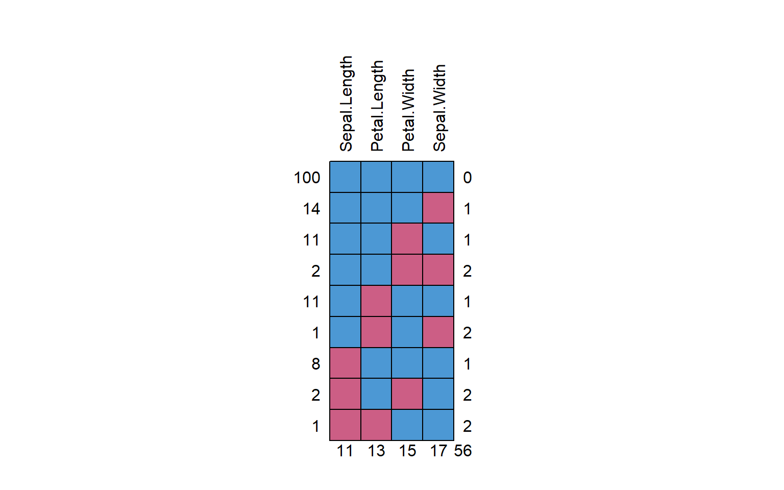
9 1.2 Multiple Imputation by Chained Equations (MICE)
MICE es uno de los métodos más utilizados en estadística aplicada para imputación múltiple. La idea es modelar cada variable con missingness condicionalmente al resto de variables.
# 1.2 Multiple Imputation by Chained Equations (MICE) ==========================# https://amices.org/mice/# Eliminamos variables categóricas para quedarnos únicamente con variables# numéricas en este ejemplo concreto.quiCat <-which(sapply(iris.mis, class) %in%c("character", "factor"))categories <-names(iris.mis)[quiCat]iris.mis2 <-subset(iris.mis, select =-c(get(categories)))# Mostramos un resumen del dataset resultante.summary(iris.mis2)
  Sepal.Length    Sepal.Width     Petal.Length    Petal.Width
 Min.   :4.300   Min.   :2.000   Min.   :1.000   Min.   :0.100
 1st Qu.:5.100   1st Qu.:2.800   1st Qu.:1.600   1st Qu.:0.300
 Median :5.700   Median :3.000   Median :4.300   Median :1.300
 Mean   :5.796   Mean   :3.065   Mean   :3.726   Mean   :1.168
 3rd Qu.:6.350   3rd Qu.:3.400   3rd Qu.:5.100   3rd Qu.:1.800
 Max.   :7.700   Max.   :4.400   Max.   :6.900   Max.   :2.500
 NA's   :11      NA's   :17      NA's   :13      NA's   :15
# Visualizamos el patrón de datos ausentes.par(mfrow =c(1, 1))md.pattern(iris.mis2, rotate.names =TRUE)
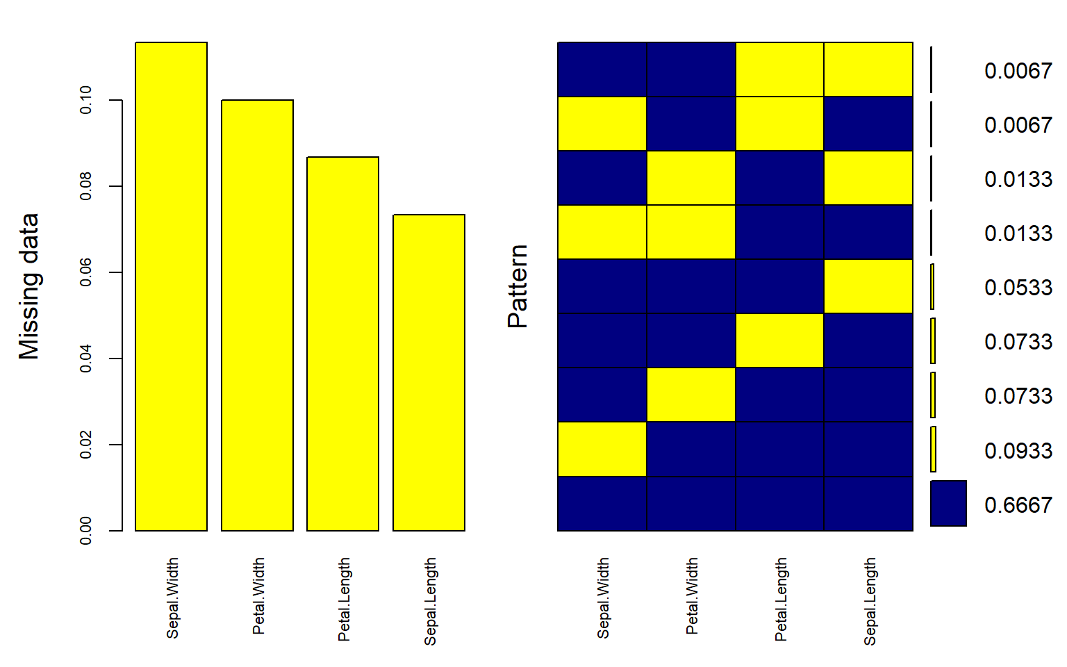
# Look the NA's with VIM packagesmice_plot <-aggr( iris.mis2,col =c("navyblue", "yellow"),numbers =TRUE,sortVars =TRUE,labels =names(iris.mis),cex.axis = .7,gap =3,ylab =c("Missing data", "Pattern"))
 Variables sorted by number of missings:
     Variable      Count
  Sepal.Width 0.11333333
  Petal.Width 0.10000000
 Petal.Length 0.08666667
 Sepal.Length 0.07333333
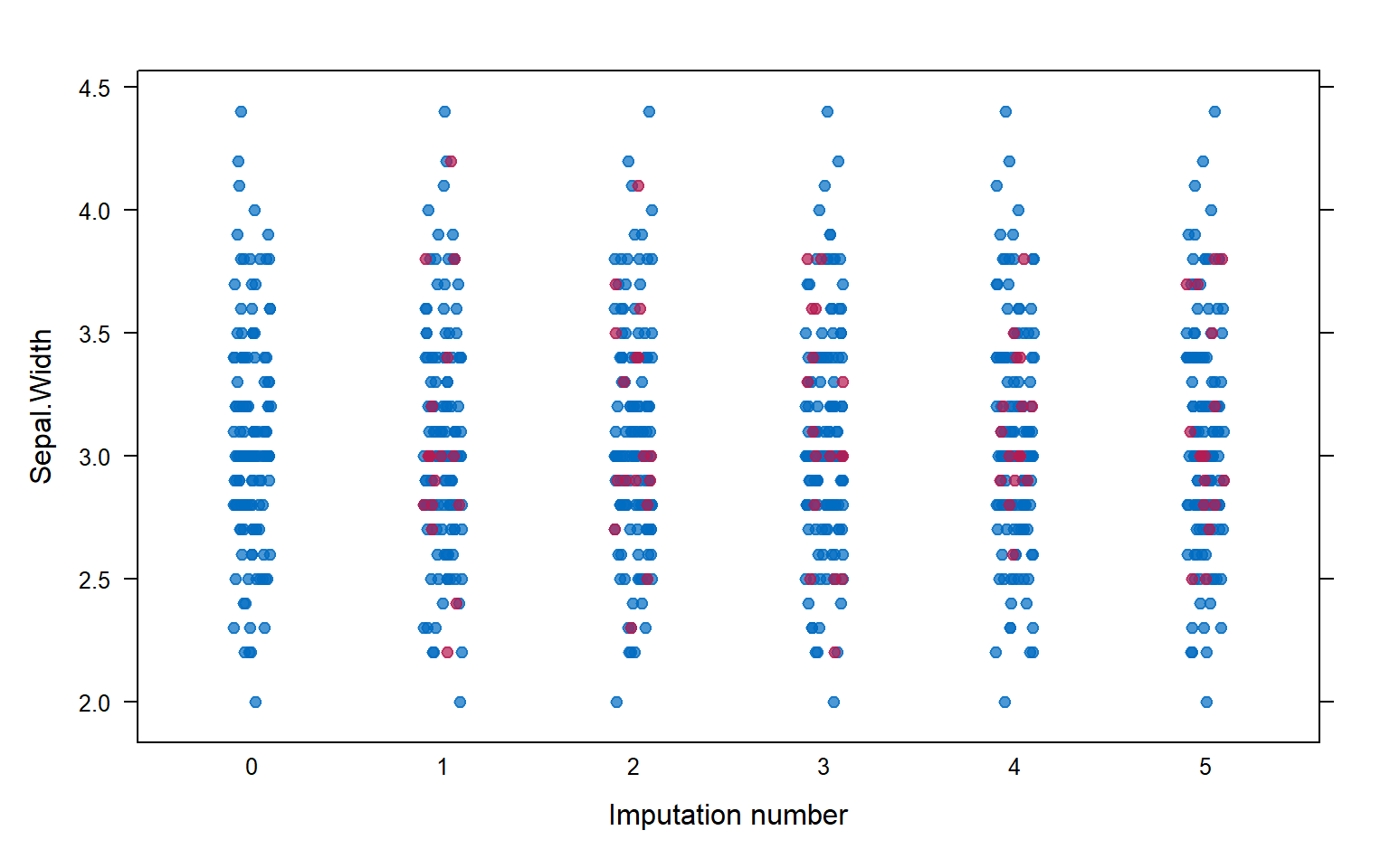
9.2 Ejecución de MICE
# Multiple impute the missing values.# m = 5 indica que generamos 5 datasets imputados.# maxit = 50 fija el número máximo de iteraciones.# method = 'pmm' usa Predictive Mean Matching.imputed_Data <-mice(iris.mis2, m =5, maxit =50, method ="pmm", seed =500)
# Inspección visual de la calidad de imputación para Sepal.Width.stripplot(imputed_Data, Sepal.Width, pch =19, xlab ="Imputation number")
# Valores imputados específicamente en Sepal.Width.imputed_Data$imp$Sepal.Width
# Recuperamos los datos completos en formato largo.completeData <- mice::complete(imputed_Data, action ="long")# Mostramos las primeras filas como inspección rápida.head(completeData)
9.3 Ejercicio propuesto
Desplegar una visualización múltiple que compare, para todas las variables numéricas del dataframe, la distribución original frente a la distribución imputada.
10 1.3 KNN
El método KNN imputa los valores faltantes utilizando observaciones cercanas en el espacio de variables. Es una técnica sencilla y efectiva cuando existe una estructura local útil en los datos.
# 1.3 KNN =====================================================================# Identificamos el tipo de cada variable.tipos <-sapply(iris.mis, class)# Seleccionamos únicamente variables numéricas e integer.varNum <-names(tipos)[which(tipos %in%c("numeric", "integer"))]# Aplicamos imputación KNN con k = 1.# Es decir, cada valor ausente se imputará usando su vecino más cercano.preProcValues <- caret::preProcess(iris.mis[, varNum], method ="knnImpute", k =1) data_knn_imputation <-predict(preProcValues, iris.mis)# Resumen del dataset imputado.summary(data_knn_imputation)
  Sepal.Length        Sepal.Width          Petal.Length
 Min.   :-1.853335   Min.   :-2.384e+00   Min.   :-1.559403
 1st Qu.:-0.862037   1st Qu.:-5.927e-01   1st Qu.:-1.259028
 Median : 0.005349   Median :-1.448e-01   Median : 0.385883
 Mean   : 0.042522   Mean   : 1.122e-05   Mean   : 0.007888
 3rd Qu.: 0.748822   3rd Qu.: 6.949e-01   3rd Qu.: 0.786383
 Max.   : 2.359682   Max.   : 2.990e+00   Max.   : 1.816241
  Petal.Width             Species
 Min.   :-1.41246   setosa    :44
 1st Qu.:-1.14799   versicolor:45
 Median : 0.17435   virginica :42
 Mean   : 0.03771   NA's      :19
 3rd Qu.: 0.83553
 Max.   : 1.76117
# Otra forma seria utilizando el paquete VIM data_knn_imputation <- VIM::kNN(iris.mis[, varNum], k =1)
# Resumen del dataset imputado.summary(data_knn_imputation)
  Sepal.Length    Sepal.Width     Petal.Length    Petal.Width
 Min.   :4.300   Min.   :2.000   Min.   :1.000   Min.   :0.100
 1st Qu.:5.100   1st Qu.:2.800   1st Qu.:1.525   1st Qu.:0.300
 Median :5.800   Median :3.000   Median :4.400   Median :1.300
 Mean   :5.825   Mean   :3.059   Mean   :3.735   Mean   :1.191
 3rd Qu.:6.400   3rd Qu.:3.300   3rd Qu.:5.100   3rd Qu.:1.800
 Max.   :7.700   Max.   :4.400   Max.   :6.900   Max.   :2.500
 Sepal.Length_imp Sepal.Width_imp Petal.Length_imp Petal.Width_imp
 Mode :logical    Mode :logical   Mode :logical    Mode :logical
 FALSE:139        FALSE:133       FALSE:137        FALSE:135
 TRUE :11         TRUE :17        TRUE :13         TRUE :15
10.1 Comparación visual con los datos reales
# Comparamos la variable Sepal.Length real frente a la imputada por KNN.newBD <-data.frame(real = iris[, "Sepal.Length"],imputed = data_knn_imputation[, "Sepal.Length"])# Reorganizamos a formato largo para representar densidades.df_long <- newBD %>%pivot_longer(cols =everything(), names_to ="Variable", values_to ="Valor")# Dibujamos la comparación de distribuciones.ggplot(df_long, aes(x = Valor, fill = Variable)) +geom_density(alpha =0.3) +labs(title ="Densidad de las dos variables",x ="Valor",y ="Densidad" ) +theme_minimal() +scale_fill_manual(values =c("blue", "red"))
10.2 Ejercicio propuesto
Desplegar una visualización múltiple que compare la imputación y los datos originales en todas las variables numéricas del dataframe.
11 1.4 missForest
missForest es un método robusto y muy utilizado cuando hay relaciones no lineales y combinaciones de variables numéricas y categóricas. Se basa en bosques aleatorios.
# 1.4 missForest ===============================================================# Imputamos los valores ausentes usando los parámetros por defecto.# variablewise = TRUE devuelve el error por variable.# verbose = TRUE muestra el progreso por consola.iris.imp <-missForest(iris.mis, variablewise =TRUE, verbose =TRUE)
# Interpretación docente:# - NRMSE (Normalized Root Mean Squared Error) se usa para variables continuas.# - PFC (Proportion of Falsely Classified) se usa para variables categóricas.
11.1 Comparación contra los datos reales
# Calculamos el error comparando:# - los datos imputados,# - el dataset con missing,# - y los datos originales completos.iris.err <-mixError(iris.imp$ximp, iris.mis, iris)iris.err
    NRMSE       PFC
0.1758295 0.0000000
# Comparamos visualmente Sepal.Length real frente a la imputada por missForest.newBD <-data.frame(real = iris[, "Sepal.Length"],imputed = iris.imp$ximp[, "Sepal.Length"])# Formato largo para la representación.df_long <- newBD %>%pivot_longer(cols =everything(), names_to ="Variable", values_to ="Valor")# Gráfico de densidades comparadas.ggplot(df_long, aes(x = Valor, fill = Variable)) +geom_density(alpha =0.3) +labs(title ="Densidad de las dos variables",x ="Valor",y ="Densidad" ) +theme_minimal() +scale_fill_manual(values =c("blue", "red"))
11.2 Ejercicio propuesto
Desplegar una visualización múltiple que compare la imputación y los datos originales en todas las variables numéricas del dataframe.
12 Extras
Cuando se trabaja con valores faltantes, en muchas ocasiones el problema no es solamente imputar, sino también detectar valores especiales que en realidad deberían considerarse NA.
Por ejemplo, en algunas bases de datos aparecen códigos como:
-99
-1
"N/A"
"Not Available"
que semánticamente representan ausencia de información.
# ==============================================================================# Extras:# When you are dealing with missing values, you might want to replace values with# a missing values (NA). This is useful in cases when you know the origin of the# data and can be certain which values should be missing. For example, you might# know that all values of “N/A”, “N A”, and “Not Available”, or -99, or -1 are# supposed to be missing.## naniar provides functions to specifically work on this type of problem using# the function replace_with_na. This function is the compliment to tidyr::replace_na,# which replaces an NA value with a specified value, whereas naniar::replace_with_na# replaces a value with an NA:## tidyr::replace_na: Missing values turns into a value (NA -> -99)# naniar::replace_with_na: Value becomes a missing value (-99 -> NA)
12.1 Ejemplo conceptual
# Ejemplo opcional de uso:# Supongamos que en una variable el valor -99 significa realmente "dato no disponible".df_example <-data.frame(x =c(1, 2, -99, 4, -99, 6))# Reemplazamos el código -99 por NA real.df_example_na <- naniar::replace_with_na(df_example, replace =list(x =-99))df_example
df_example_na
13 Conclusiones docentes
A nivel pedagógico, este guion permite mostrar una progresión natural:
Generar y detectar missingness.
Visualizar patrones de ausencia.
Aplicar imputaciones simples como referencia.
Evolucionar hacia métodos más robustos como MICE, KNN y missForest.
Comparar distribuciones para evaluar si la imputación distorsiona o preserva la estructura de los datos.
En términos metodológicos:
las imputaciones por media son fáciles de explicar pero pueden sesgar la varianza,
las imputaciones condicionadas por grupo introducen estructura supervisada útil,
MICE ofrece una aproximación estadísticamente sólida,
KNN aprovecha vecindad local,
missForest suele rendir muy bien cuando hay no linealidades y mixtura de tipos.
Aquesta web està creada por Dante Conti y Sergi Ramírez, (c) 2026
Ejecutar el código
---title: "Preprocessing: Imputación de datos faltantes"subtitle: "Material docente en Quarto a partir del script original"author: - "Sergi Ramírez" - "Dante Conti"format: html: theme: cosmo toc: true toc-depth: 3 number-sections: true code-fold: false code-tools: true df-print: paged fig-width: 8 fig-height: 5execute: echo: true warning: false message: false cache: falselang: eseditor: visual---# IntroducciónEste documento docente presenta, de forma estructurada y comentada, distintos métodos de **imputación de datos faltantes** en R.Se ha respetado al máximo la organización del script original, incorporando:- explicación conceptual antes de cada bloque,- comentarios detallados dentro del código,- separación por apartados para facilitar la docencia,- y una estructura adecuada para usar directamente en **Quarto**.## Objetivos docentesAl finalizar este material, el estudiante debería poder:1. generar artificialmente valores perdidos,2. explorar patrones de missingness,3. distinguir entre técnicas básicas y avanzadas de imputación,4. aplicar métodos como **media**, **aregImpute**, **MI**, **MICE**, **KNN** y **missForest**,5. comparar distribuciones originales e imputadas.------------------------------------------------------------------------# Carga de libreríasEn este primer bloque cargamos todos los paquetes necesarios para trabajar con visualización, exploración de valores perdidos e imputación.```{r}# Carreguem les llibreries =====================================================# Vector con los paquetes que vamos a necesitar durante toda la práctica.# Incluye paquetes para:# - visualización (ggplot2, plotly, visdata, VIM)# - manipulación de datos (dplyr, tidyverse)# - análisis de missingness (naniar, mi)# - imputación (Hmisc, mice, DMwR, missForest)list.of.packages <-c("ggplot2", "plotly", "dplyr", "tidyverse", "naniar","mi", "Hmisc", "mice", "pool", "VIM", "missForest", "RANN", "caret")# Detectamos qué paquetes no están instalados en el sistema.new.packages <- list.of.packages[!(list.of.packages %in%installed.packages()[, "Package"])]# Si falta alguno, lo instalamos automáticamente.if (length(new.packages) >0) {install.packages(new.packages)}# Cargamos todos los paquetes en memoria.lapply(list.of.packages, require, character.only =TRUE)# Limpiamos objetos auxiliares que ya no necesitamos y lanzamos el recolector# de basura para liberar memoria.rm(list.of.packages, new.packages)gc()```------------------------------------------------------------------------# Generación de datos con valores perdidosPara practicar métodos de imputación, primero generamos una versión incompleta del conjunto de datos `iris`, introduciendo un 10% de valores ausentes de forma artificial.```{r}# Generate data with NA's ======================================================# Generamos una copia del dataset iris con aproximadamente un 10% de valores NA.# La función prodNA del paquete missForest introduce missing values de forma# artificial para que podamos practicar imputación.iris.mis <- missForest::prodNA(iris, noNA =0.1)# Otras formas de crear valores ausentes artificialmente en un dataframe:# iris.mis <- mi::create.missing(iris, pct.mis = 10)# Mostramos un resumen básico del dataset con NA para inspeccionar su estructura.summary(iris.mis)```------------------------------------------------------------------------# Little TestUna cuestión importante en datos faltantes es entender si los NA aparecen completamente al azar o siguen algún patrón. Para ello usamos el test MCAR.```{r}# Little Test ==================================================================# Aplicamos el test MCAR (Missing Completely At Random).# Este contraste ayuda a evaluar si los datos faltantes se generan de manera# completamente aleatoria.naniar::mcar_test(iris.mis)# Interpretación conceptual:# - Si el p-valor es pequeño, rechazamos que los missing sean completamente aleatorios.# - Si el p-valor no es pequeño, no tenemos evidencia para rechazar MCAR.# Nota importante docente:# En el script original aparece el comentario:# "If the test p-value is less than 0 this means..."# Lo correcto estadísticamente sería hablar de un p-valor bajo, por ejemplo < 0.05.```------------------------------------------------------------------------# Patrones descriptivos de valores perdidos en una base de datosAntes de imputar, conviene **visualizar** y **describir** los patrones de ausencia. Esto ayuda a detectar si hay variables particularmente afectadas o relaciones entre missingness y otras variables.## Exploración visual de missingness```{r}# Descriptive NA's patterns in a databases =====================================# Cargamos explícitamente visdat para sus funciones de visualización.library(visdat)# Visualizamos el tipo de dato y la presencia de NA en airquality.vis_dat(airquality)# Visualizamos el tipo de dato y la presencia de NA en iris.mis.vis_dat(iris.mis)# Representación específica de valores perdidos en airquality.vis_miss(airquality)# Representación específica de valores perdidos en iris.mis.vis_miss(iris.mis)```## Relación entre valores perdidos y variables numéricas```{r}# Gráfico básico de dispersión sin destacar missingness.ggplot(airquality, aes(x = Solar.R, y = Ozone)) +geom_point()# Gráfico de dispersión destacando las observaciones con missingness.ggplot(airquality, aes(x = Solar.R, y = Ozone)) +geom_miss_point()# Añadimos facetado por mes para observar si el patrón de NA cambia según el mes.ggplot(airquality, aes(x = Solar.R, y = Ozone)) +geom_miss_point() +facet_wrap(~Month)# Mismo gráfico anterior pero con tema oscuro para enfatizar la visualización.ggplot(airquality, aes(x = Solar.R, y = Ozone)) +geom_miss_point() +facet_wrap(~Month) +theme_dark()```## Visualización del número de missings por variable```{r}# Visualizamos cuántos NA tiene cada variable.gg_miss_var(airquality) +labs(y ="Look at all the missing ones")```## Sombra de missingness y resumen por grupos```{r}# Detect NA in Dataframe =======================================================# Creamos un shadow matrix: añade variables auxiliares con sufijo _NA que indican# si el valor original era NA o no.aq_shadow <-bind_shadow(airquality)# Calculamos estadísticas descriptivas de Solar.R separando los registros según# si Ozone es NA o no.airquality %>%bind_shadow() %>%group_by(Ozone_NA) %>%summarise_at(.vars ="Solar.R",.funs =c("mean", "sd", "var", "min", "max"),na.rm =TRUE )# Representamos la distribución de la temperatura diferenciando los casos en los# que Ozone está ausente de aquellos en los que no lo está.ggplot(aq_shadow, aes(x = Temp, colour = Ozone_NA)) +geom_density()```## Estadísticos de missingness```{r}# Extract statistics with NAs in Data Frame ====================================# Proporción de casos (filas) que contienen algún NA.prop_miss_case(airquality)# Porcentaje de casos con NA.pct_miss_case(airquality)# Resumen por fila del patrón de missingness.miss_case_summary(airquality)# Tabla de frecuencia del número de missings por fila.miss_case_table(airquality)# Proporción de missings por variable.prop_miss_var(airquality)# Porcentaje de missings por variable.pct_miss_var(airquality)# Resumen de missingness por variable.miss_var_summary(airquality)# Tabla de frecuencia de missings por variable.miss_var_table(airquality)```------------------------------------------------------------------------# 1.1 Imputación básicaEn este apartado se ilustran técnicas sencillas de imputación, útiles para comprender la lógica general aunque normalmente insuficientes en contextos reales complejos.## Imputación con la media y con valores aleatorios```{r}# 1.1 Basic Imputation ========================================================# Imputamos los NA de Sepal.Length usando la media de la variable.# La función impute del paquete Hmisc devuelve una versión imputada de la variable.iris.mis[, "imputed_Sepal.Length"] <-with(iris.mis, impute(Sepal.Length, mean))# Imputamos los NA de Sepal.Length usando valores aleatorios observados.iris.mis[, "imputed_Sepal.Length2"] <-with(iris.mis, impute(Sepal.Length, "random"))# Nota docente:# De forma análoga se podrían usar estrategias como min, max o median.# Reestructuramos los datos a formato largo para comparar distribuciones.df_long <- iris.mis %>%select(Sepal.Length, imputed_Sepal.Length, imputed_Sepal.Length2) %>%pivot_longer(cols =everything(), names_to ="Variable", values_to ="Valor")# Representamos la densidad de la variable original y de las variables imputadas.ggplot(df_long, aes(x = Valor, fill = Variable)) +geom_density(alpha =0.3) +labs(title ="Densidad de las tres variables",x ="Valor",y ="Densidad" ) +theme_minimal() +scale_fill_manual(values =c("blue", "red", "green"))# Eliminamos las variables auxiliares para no contaminar el dataframe original.iris.mis[, c("imputed_Sepal.Length", "imputed_Sepal.Length2")] <-NULL```## Imputación con `aregImpute``aregImpute` implementa una imputación basada en modelos aditivos flexibles y múltiples simulaciones. Aquí se aplica sobre todas las variables del dataset.```{r}# ------------------------------------------------------------------------------# using argImpute# Ajustamos el modelo de imputación.# n.impute = 5 indica que se generan 5 imputaciones para los valores ausentes.impute_arg <-aregImpute(~ Sepal.Length + Sepal.Width + Petal.Length + Petal.Width + Species,data = iris.mis,n.impute =5)# Mostramos el objeto resultante para inspeccionar la imputación.impute_arg# Revisamos específicamente las imputaciones generadas para Sepal.Length.impute_arg$imputed$Sepal.Length# Calculamos la media de las 5 imputaciones para cada observación ausente.imputed_Sepal.Length <-rowMeans(impute_arg$imputed$Sepal.Length)# Creamos una nueva variable partiendo de la variable real original.new_var_imputed <- iris$Sepal.Length# Sustituimos únicamente las posiciones que tenían NA por la media imputada.new_var_imputed[as.numeric(names(imputed_Sepal.Length))] <- imputed_Sepal.Length# Comparamos la distribución real frente a la imputada.newBD <-data.frame(real = iris[, "Sepal.Length"], imputed = new_var_imputed)df_long <- newBD %>%pivot_longer(cols =everything(), names_to ="Variable", values_to ="Valor")ggplot(df_long, aes(x = Valor, fill = Variable)) +geom_density(alpha =0.3) +labs(title ="Densidad de las dos variables",x ="Valor",y ="Densidad" ) +theme_minimal() +scale_fill_manual(values =c("blue", "red"))```------------------------------------------------------------------------# 1.1.1 Multiple Iterative Regression Imputation (MI method)Este bloque usa el paquete `mi`, que implementa imputación múltiple mediante aproximaciones iterativas basadas en modelos probabilísticos.```{r}# 1.1.1 Multiple Iterative Regression Imputation (MI method) -------------------# Ejecutamos la imputación múltiple con una semilla fija para garantizar# reproducibilidad.mi_data <-mi(iris.mis, seed =335)# Resumen del modelo de imputación.summary(mi_data)# Gráficos diagnósticos del proceso de imputación.plot(mi_data)# Evitamos que R pregunte entre gráficos cuando hay múltiples paneles.par(ask =FALSE)# Revisamos la estructura interna del objeto de imputación.mi_data@data```------------------------------------------------------------------------# 1.1.2 Media condicionada por variable objetivoAquí se aplica una estrategia simple pero útil en docencia: imputar con la **media del grupo**, definida por una variable objetivo o categórica, en este caso `Species`.```{r}# 1.1.2 MEAN WITH TARGET VARS --------------------------------------------------# Definimos la variable objetivo o de agrupación.target <-"Species"# Construimos un dataset sin la variable target para introducir NA únicamente# en las variables predictoras.data <-subset(iris, select =-c(get(target)))# Generamos valores ausentes de forma artificial.data <-prodNA(data, noNA =0.1)# Recuperamos la variable target original.data$Species <- iris[, target]# Identificamos qué variables debemos imputar: todas excepto la target.varImp <-colnames(data)[which(!colnames(data) %in% target)]# Calculamos la media de cada variable numérica dentro de cada grupo de Species.means <-aggregate(data[, varImp], list(data[, target]), mean, na.rm =TRUE)# Imputamos los valores ausentes usando la media de su grupo.for (c in varImp) {for (g in means[, "Group.1"]) {# Condición lógica: filas que pertenecen al grupo g. cond <- data[, target] == g# Detectamos los NA de la variable c dentro de ese grupo. na_index <-is.na(data[, c]) & cond# Sustituimos cada NA por la media del grupo correspondiente. data[na_index, c] <- means[means[, "Group.1"] == g, c] }}# Resumen del dataset imputado.summary(data)```## Comparación visual entre original e imputado```{r}# Marcamos el origen de cada dataset para poder compararlos visualmente.iris[, "Tipo"] <-"original"data[, "Tipo"] <-"imputed"# Fusionamos ambos dataframes en uno solo.data_long <-bind_rows(iris, data)# Seleccionamos únicamente las variables numéricas para representar densidades.cols_numeric <-names(data_long)[sapply(data_long, is.numeric) &names(data_long) !="Tipo"]# Pasamos a formato largo para facetar un gráfico por variable.data_long <- data_long %>%pivot_longer(cols =all_of(cols_numeric), names_to ="Variable", values_to ="Valor")# Representamos la comparación de distribuciones por variable.ggplot(data_long, aes(x = Valor, fill = Tipo)) +geom_density(alpha =0.3) +facet_wrap(~Variable, scales ="free") +labs(title ="Comparación de Distribuciones: Original vs Imputado",x ="Valor",y ="Densidad" ) +theme_minimal() +scale_fill_manual(values =c("blue", "red"))# Nota docente:# En el script original aparece esta línea:# iris.mis[, "Tipo"] <- NULL# Sin embargo, la columna Tipo se añadió a iris y data, no a iris.mis.# Por coherencia, eliminamos la columna Tipo del dataset iris original.iris[, "Tipo"] <-NULL```------------------------------------------------------------------------# 1.2 Multiple Imputation by Chained Equations (MICE)MICE es uno de los métodos más utilizados en estadística aplicada para imputación múltiple. La idea es modelar cada variable con missingness condicionalmente al resto de variables.```{r}# 1.2 Multiple Imputation by Chained Equations (MICE) ==========================# https://amices.org/mice/# Eliminamos variables categóricas para quedarnos únicamente con variables# numéricas en este ejemplo concreto.quiCat <-which(sapply(iris.mis, class) %in%c("character", "factor"))categories <-names(iris.mis)[quiCat]iris.mis2 <-subset(iris.mis, select =-c(get(categories)))# Mostramos un resumen del dataset resultante.summary(iris.mis2)# Visualizamos el patrón de datos ausentes.par(mfrow =c(1, 1))md.pattern(iris.mis2, rotate.names =TRUE)```## Visualización del patrón con VIM```{r}# Look the NA's with VIM packagesmice_plot <-aggr( iris.mis2,col =c("navyblue", "yellow"),numbers =TRUE,sortVars =TRUE,labels =names(iris.mis),cex.axis = .7,gap =3,ylab =c("Missing data", "Pattern"))```## Ejecución de MICE```{r}# Multiple impute the missing values.# m = 5 indica que generamos 5 datasets imputados.# maxit = 50 fija el número máximo de iteraciones.# method = 'pmm' usa Predictive Mean Matching.imputed_Data <-mice(iris.mis2, m =5, maxit =50, method ="pmm", seed =500)# Resumen del objeto de imputación.summary(imputed_Data)# Inspección visual de la calidad de imputación para Sepal.Width.stripplot(imputed_Data, Sepal.Width, pch =19, xlab ="Imputation number")# Valores imputados específicamente en Sepal.Width.imputed_Data$imp$Sepal.Width# Recuperamos los datos completos en formato largo.completeData <- mice::complete(imputed_Data, action ="long")# Mostramos las primeras filas como inspección rápida.head(completeData)```## Ejercicio propuesto> Desplegar una visualización múltiple que compare, para todas las variables numéricas del dataframe, la distribución original frente a la distribución imputada.------------------------------------------------------------------------# 1.3 KNNEl método KNN imputa los valores faltantes utilizando observaciones cercanas en el espacio de variables. Es una técnica sencilla y efectiva cuando existe una estructura local útil en los datos.```{r}# 1.3 KNN =====================================================================# Identificamos el tipo de cada variable.tipos <-sapply(iris.mis, class)# Seleccionamos únicamente variables numéricas e integer.varNum <-names(tipos)[which(tipos %in%c("numeric", "integer"))]# Aplicamos imputación KNN con k = 1.# Es decir, cada valor ausente se imputará usando su vecino más cercano.preProcValues <- caret::preProcess(iris.mis[, varNum], method ="knnImpute", k =1) data_knn_imputation <-predict(preProcValues, iris.mis)# Resumen del dataset imputado.summary(data_knn_imputation)# Otra forma seria utilizando el paquete VIM data_knn_imputation <- VIM::kNN(iris.mis[, varNum], k =1)# Resumen del dataset imputado.summary(data_knn_imputation)```## Comparación visual con los datos reales```{r}# Comparamos la variable Sepal.Length real frente a la imputada por KNN.newBD <-data.frame(real = iris[, "Sepal.Length"],imputed = data_knn_imputation[, "Sepal.Length"])# Reorganizamos a formato largo para representar densidades.df_long <- newBD %>%pivot_longer(cols =everything(), names_to ="Variable", values_to ="Valor")# Dibujamos la comparación de distribuciones.ggplot(df_long, aes(x = Valor, fill = Variable)) +geom_density(alpha =0.3) +labs(title ="Densidad de las dos variables",x ="Valor",y ="Densidad" ) +theme_minimal() +scale_fill_manual(values =c("blue", "red"))```## Ejercicio propuesto> Desplegar una visualización múltiple que compare la imputación y los datos originales en todas las variables numéricas del dataframe.------------------------------------------------------------------------# 1.4 missForest`missForest` es un método robusto y muy utilizado cuando hay relaciones no lineales y combinaciones de variables numéricas y categóricas. Se basa en bosques aleatorios.```{r}# 1.4 missForest ===============================================================# Imputamos los valores ausentes usando los parámetros por defecto.# variablewise = TRUE devuelve el error por variable.# verbose = TRUE muestra el progreso por consola.iris.imp <-missForest(iris.mis, variablewise =TRUE, verbose =TRUE)# Consultamos el dataframe imputado final.iris.imp$ximp# Revisamos el error de imputación out-of-bag.iris.imp$OOBerror# Interpretación docente:# - NRMSE (Normalized Root Mean Squared Error) se usa para variables continuas.# - PFC (Proportion of Falsely Classified) se usa para variables categóricas.```## Comparación contra los datos reales```{r}# Calculamos el error comparando:# - los datos imputados,# - el dataset con missing,# - y los datos originales completos.iris.err <-mixError(iris.imp$ximp, iris.mis, iris)iris.err# Comparamos visualmente Sepal.Length real frente a la imputada por missForest.newBD <-data.frame(real = iris[, "Sepal.Length"],imputed = iris.imp$ximp[, "Sepal.Length"])# Formato largo para la representación.df_long <- newBD %>%pivot_longer(cols =everything(), names_to ="Variable", values_to ="Valor")# Gráfico de densidades comparadas.ggplot(df_long, aes(x = Valor, fill = Variable)) +geom_density(alpha =0.3) +labs(title ="Densidad de las dos variables",x ="Valor",y ="Densidad" ) +theme_minimal() +scale_fill_manual(values =c("blue", "red"))```## Ejercicio propuesto> Desplegar una visualización múltiple que compare la imputación y los datos originales en todas las variables numéricas del dataframe.------------------------------------------------------------------------# ExtrasCuando se trabaja con valores faltantes, en muchas ocasiones el problema no es solamente imputar, sino también **detectar valores especiales que en realidad deberían considerarse NA**.Por ejemplo, en algunas bases de datos aparecen códigos como:- `-99`- `-1`- `"N/A"`- `"Not Available"`que semánticamente representan ausencia de información.```{r}# ==============================================================================# Extras:# When you are dealing with missing values, you might want to replace values with# a missing values (NA). This is useful in cases when you know the origin of the# data and can be certain which values should be missing. For example, you might# know that all values of “N/A”, “N A”, and “Not Available”, or -99, or -1 are# supposed to be missing.## naniar provides functions to specifically work on this type of problem using# the function replace_with_na. This function is the compliment to tidyr::replace_na,# which replaces an NA value with a specified value, whereas naniar::replace_with_na# replaces a value with an NA:## tidyr::replace_na: Missing values turns into a value (NA -> -99)# naniar::replace_with_na: Value becomes a missing value (-99 -> NA)```## Ejemplo conceptual```{r}# Ejemplo opcional de uso:# Supongamos que en una variable el valor -99 significa realmente "dato no disponible".df_example <-data.frame(x =c(1, 2, -99, 4, -99, 6))# Reemplazamos el código -99 por NA real.df_example_na <- naniar::replace_with_na(df_example, replace =list(x =-99))df_exampledf_example_na```------------------------------------------------------------------------# Conclusiones docentesA nivel pedagógico, este guion permite mostrar una progresión natural:1. **Generar y detectar missingness**.2. **Visualizar patrones de ausencia**.3. **Aplicar imputaciones simples** como referencia.4. **Evolucionar hacia métodos más robustos** como MICE, KNN y missForest.5. **Comparar distribuciones** para evaluar si la imputación distorsiona o preserva la estructura de los datos.En términos metodológicos:- las imputaciones por media son fáciles de explicar pero pueden sesgar la varianza,- las imputaciones condicionadas por grupo introducen estructura supervisada útil,- MICE ofrece una aproximación estadísticamente sólida,- KNN aprovecha vecindad local,- missForest suele rendir muy bien cuando hay no linealidades y mixtura de tipos.------------------------------------------------------------------------# Bibliografía- <http://naniar.njtierney.com/articles/replace-with-na.html>- <https://cran.r-project.org/web/packages/visdat/vignettes/using_visdat.html>- <https://cran.r-project.org/web/packages/DMwR2/DMwR2.pdf>- <https://ltorgo.github.io/DMwR2/RintroDM.html#data_pre-processing>- <https://www.rdocumentation.org/packages/DMwR/versions/0.4.1/topics/knnImputation>